
NICS Spectroscopic Modes
Slits |
|||||||||||||||||||||||||||||||||||||||||||||||||||||||||||||||||||||
|
Long slit spectroscopic observations are performed by inserting a slit at the entrance focal plane and a disperser (grism or prism) in the collimated beam. The table here lists the slits available in NICS which, thanks to the refurbishment works of Feb-Mar 2003, have now a very stable and repeatable positioning. All spectroscopic modes make use of the LF camera with a scale of 0.25"/pixel. |
||||||||||||||||||||||||||||||||||||||||||||||||||||||||||||||||||||
Dispersers |
|||||||||||||||||||||||||||||||||||||||||||||||||||||||||||||||||||||
|
The instrument is equipped with one prism and a number of grism dispersers
whose main characteristics are displayed in this
figure and listed in the table on the left.
Note that the grisms have a fairly constant dispersion (Å/pix) throughout
the spectrum and, therefore, their resolving power increases going towards the red.
The Amici prism, on the contrary, delivers a spectrum with a quasi-constant
resolving power and, therefore, its dispersion varies by more than a factor
of 3 over its spectral range. |
||||||||||||||||||||||||||||||||||||||||||||||||||||||||||||||||||||
Wavelength calibration and sky spectra |
|||||||||||||||||||||||||||||||||||||||||||||||||||||||||||||||||||||
|
GRISMS An accurate wavelength calibration
and a proper rectification of the (curved) slit images can be achieved
using a two dimensional polynomial of 3rd or 4rd degree in the dispersion (X)
direction and 2nd or 3rd degree in the spatial (Y) direction.
All the spectra are correctly oriented (i.e. blue is to the left),
click on the rainbows in the table to get a view
of the bi-dimensional spectra.
The labelled wavelengths are in air and refer to lines which are bright
and isolated.
Please note that while the Argon lamp provides good calibration
frames for basically all the grisms, the Xenon spectrum is less rich of lines
in the K band.
Examples of wavelength calibrated spectra
in the form of ascii files can be also found by clicking on the grism name
in the table. AMICI PRISM The spectrum is flipped (i.e. blue is to the right) and occupies only the central part of the array. Due to the very low resolution, virtually all the Ar/Xe lines are blended and cannot be easily used for standard reduction procedures. For this reason, wavelength calibration is normally performed using a look-up table which is based on the theoretical dispersion predicted by ray-tracing and adjusted to best fit the observed spectra of calibration sources. Slit curvature is very modest and evident only in the reddest part of the spectrum, it can be usually neglected. |
||||||||||||||||||||||||||||||||||||||||||||||||||||||||||||||||||||
Flats |
|||||||||||||||||||||||||||||||||||||||||||||||||||||||||||||||||||||
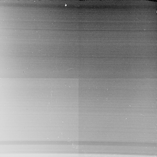 Example of an halogen exposure with the IJ grism |
The main reason why one needs a flat is to correct
the "granulation" (not-uniform pixel-to-pixel response) which is
instrinsic to the array and can be corrected for by
using deep halogen lamps exposures taken within several days
from the observations.
|
||||||||||||||||||||||||||||||||||||||||||||||||||||||||||||||||||||
Performances
The observational performances for spectroscopy can
be estimated using our Exposure Calculator
which is based on the measured zero points, backgrounds, array
noise and yields the average s/n ratio achievable for a source with a given magnitude or,
alternatively, the time necessary to achieve a chosen s/n for a given source property.
Please note that the program assumes a maximum on-chip integration time
of 900 sec and provides just a representative figure for
the central wavelength of each photometric band for which a spectral-averaged
background level is also adopted. The actual s/n varies significantly with wavelength
following the instrumental efficiency curve and the spectral distribution of the sky emission.
The limiting fluxes for line detection can be roughly estimated by multiplying the flux per wavelength unit corresponding to a given object magnitude, times the line width which, for unresolved lines, is set by the slit width (in pixels) times the dispersion (Å/pix).
For any comments please contact Vania Lorenzi.